Logit Ableitung Rechner
Online Rechner für die Derivative der Logit-Funktion
Geben Sie die Wahrscheinlichkeit (p) zwischen 0 und 1 ein und klicken Sie auf Berechnen um die Ableitung der Logit-Funktion zu ermitteln. Die Logit-Ableitung ist fundamental für die statistische Inferenz und hat ihr Minimum bei p=0.5 mit dem Wert 4.
💡 Logit Ableitung
\(\text{logit}'(p) = \frac{d}{dp}\ln\left(\frac{p}{1-p}\right) = \frac{1}{p(1-p)}\)
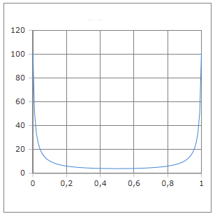
Die U-förmige Kurve der Logit-Ableitung mit Minimum bei p=0.5
Die Logit-Ableitung verstehen
Die Ableitung der Logit-Funktion ist von zentraler Bedeutung in der statistischen Modellierung und logistischen Regression. Sie hat eine charakteristische U-förmige Kurve mit ihrem Minimum bei p=0.5 und dem Wert 4. Die Funktion logit'(p) = 1/(p·(1-p)) repräsentiert die Fisher-Information für die Bernoulli-Verteilung und ist fundamental für Konfidenzintervalle und Hypothesentests.
📈 Grundformeln
Verschiedene Darstellungen:
📊 Eigenschaften
- • Minimum: logit'(0.5) = 4
- • Symmetrisch um p=0.5
- • U-förmige Kurve
- • Divergenz bei p→0 und p→1
🔬 Anwendungen
- • Fisher-Information-Matrix
- • Cramér-Rao-Schranke
- • Asymptotische Varianz
- • Konfidenzintervalle
⚠️ Besonderheiten
- • Divergenz an Grenzen
- • Numerische Instabilität
- • Varianz-Stabilisierung
- • Delta-Methode relevant
Mathematische Herleitung
📈 Ableitung der Logit-Funktion
Schritt-für-Schritt Herleitung:
\[\text{Gegeben: } \text{logit}(p) = \ln\left(\frac{p}{1-p}\right)\] \[\text{Umschreibung: } \text{logit}(p) = \ln(p) - \ln(1-p)\] \[\text{Ableitung nach p:}\] \[\frac{d}{dp}\text{logit}(p) = \frac{d}{dp}[\ln(p) - \ln(1-p)]\] \[= \frac{1}{p} - \frac{1}{1-p} \cdot (-1) = \frac{1}{p} + \frac{1}{1-p}\] \[= \frac{1-p+p}{p(1-p)} = \frac{1}{p(1-p)}\]
🔄 Fisher-Information-Beziehung
Verbindung zur statistischen Inferenz:
\[\text{Score-Funktion: } S(p) = \frac{\partial}{\partial p}\ln L(p)\] \[\text{Fisher-Information: } I(p) = E[S(p)^2] = -E\left[\frac{\partial^2}{\partial p^2}\ln L(p)\right]\] \[\text{Für Bernoulli: } I(p) = \frac{1}{p(1-p)} = \text{logit}'(p)\] \[\text{Cramér-Rao: } \text{Var}(\hat{p}) \geq \frac{1}{I(p)} = p(1-p)\]
📊 Charakteristische Werte
Wichtige Punkte der Logit-Ableitung:
\[\text{Minimum bei } p = 0{,}5: \quad \text{logit}'(0{,}5) = \frac{1}{0{,}5 \cdot 0{,}5} = 4\] \[\text{Symmetrie: } \text{logit}'(p) = \text{logit}'(1-p)\] \[\text{Grenzwerte: } \lim_{p \to 0^+} \text{logit}'(p) = +\infty, \quad \lim_{p \to 1^-} \text{logit}'(p) = +\infty\] \[\text{Konvexität: } \text{logit}''(p) = \frac{2p-1}{p^2(1-p)^2} > 0 \text{ für } p \neq 0{,}5\]
Praktische Berechnungsbeispiele
📝 Beispiel 1: Konfidenzintervall berechnen
Aufgabe: 95%-Konfidenzintervall für logistische Regression
Gegeben: Geschätzte Wahrscheinlichkeit p̂ = 0.3, n = 100
Berechnung:
\[\text{Logit-Ableitung: } \text{logit}'(0{,}3) = \frac{1}{0{,}3 \cdot 0{,}7} = \frac{1}{0{,}21} \approx 4{,}76\] \[\text{Asymptotische Varianz: } \text{Var}(\text{logit}(\hat{p})) \approx \frac{1}{n \cdot p(1-p)} = \frac{4{,}76}{100} = 0{,}048\] \[\text{Standard-Fehler: } SE = \sqrt{0{,}048} \approx 0{,}218\] \[\text{95\%-KI für logit: } \text{logit}(0{,}3) \pm 1{,}96 \cdot 0{,}218\] \[= -0{,}847 \pm 0{,}428 = [-1{,}275, -0{,}419]\]
Rücktransformation: KI für p: [0.218, 0.397]
📝 Beispiel 2: Delta-Methode
Aufgabe: Asymptotische Verteilung von g(p̂)
Szenario: Transformation einer Wahrscheinlichkeitsschätzung
Berechnung:
\[\text{Sei } g(p) = \text{logit}(p), \quad \hat{p} \sim N\left(p, \frac{p(1-p)}{n}\right)\] \[\text{Delta-Methode: } g(\hat{p}) \sim N\left(g(p), [g'(p)]^2 \cdot \frac{p(1-p)}{n}\right)\] \[\text{Mit } g'(p) = \text{logit}'(p) = \frac{1}{p(1-p)}:\] \[\text{logit}(\hat{p}) \sim N\left(\text{logit}(p), \frac{1}{np(1-p)}\right)\] \[\text{Varianz-Stabilisierung erreicht!}\]
Vorteil: Konstante asymptotische Varianz unabhängig von p
📝 Beispiel 3: Numerische Stabilität
Aufgabe: Berechnung bei extremen Wahrscheinlichkeiten
Problem: p = 0.0001 oder p = 0.9999
Berechnung:
\[\text{Extreme Werte: } p_1 = 0{,}0001, \quad p_2 = 0{,}9999\] \[\text{logit}'(0{,}0001) = \frac{1}{0{,}0001 \cdot 0{,}9999} \approx 10{.}001\] \[\text{logit}'(0{,}9999) = \frac{1}{0{,}9999 \cdot 0{,}0001} \approx 10{.}001\] \[\text{Problem: Numerische Instabilität bei } p \to 0 \text{ oder } p \to 1\] \[\text{Lösung: Clipping auf } [10^{-6}, 1-10^{-6}]\]
Praxis: Verwendung numerisch stabiler Implementierungen
Statistische Anwendungen
📊 Logistische Regression
Verwendung in der Maximum-Likelihood-Schätzung:
\[\text{Likelihood: } L(\boldsymbol{\beta}) = \prod_{i=1}^n p_i^{y_i}(1-p_i)^{1-y_i}\] \[\text{Log-Likelihood: } \ell(\boldsymbol{\beta}) = \sum_{i=1}^n [y_i \ln p_i + (1-y_i)\ln(1-p_i)]\] \[\text{Score: } \frac{\partial\ell}{\partial\beta_j} = \sum_{i=1}^n (y_i - p_i) x_{ij}\] \[\text{Hessian: } \frac{\partial^2\ell}{\partial\beta_j\partial\beta_k} = -\sum_{i=1}^n p_i(1-p_i) x_{ij}x_{ik}\]
📈 Newton-Raphson-Verfahren
Optimierung mit der Logit-Ableitung:
\[\text{Update-Regel: } \boldsymbol{\beta}^{(t+1)} = \boldsymbol{\beta}^{(t)} - [\mathbf{H}^{(t)}]^{-1}\mathbf{s}^{(t)}\] \[\text{Wobei: } H_{jk} = \sum_{i=1}^n \text{logit}'(p_i) \cdot p_i(1-p_i) \cdot x_{ij}x_{ik}\] \[\text{Gewichte: } w_i = p_i(1-p_i) = \frac{1}{\text{logit}'(p_i)}\] \[\text{IRLS: Iteratively Reweighted Least Squares}\]
🎯 Wald-Test und Konfidenzintervalle
Asymptotische Tests mit Fisher-Information:
\[\text{Wald-Statistik: } W = \frac{(\hat{\beta}_j - \beta_{j0})^2}{\widehat{\text{Var}}(\hat{\beta}_j)} \sim \chi^2_1\] \[\text{Asymptotische Varianz: } \text{Var}(\hat{\beta}_j) = [\mathbf{I}(\boldsymbol{\beta})]^{-1}_{jj}\] \[\text{Konfidenzintervall: } \hat{\beta}_j \pm z_{\alpha/2} \sqrt{\widehat{\text{Var}}(\hat{\beta}_j)}\] \[\text{Likelihood-Ratio: } -2[\ell(\boldsymbol{\beta}_0) - \ell(\hat{\boldsymbol{\beta}})] \sim \chi^2_p\]
📊 Ableitungswerte-Tabelle
| p | logit(p) | logit'(p) | SE(logit) | Interpretation |
|---|---|---|---|---|
| 0.05 | -2.944 | 21.053 | 0.145 | Hohe Unsicherheit |
| 0.10 | -2.197 | 11.111 | 0.105 | Mittlere Unsicherheit |
| 0.25 | -1.099 | 5.333 | 0.073 | Moderate Unsicherheit |
| 0.50 | 0.000 | 4.000 | 0.063 | Minimale Unsicherheit |
| 0.75 | 1.099 | 5.333 | 0.073 | Moderate Unsicherheit |
| 0.90 | 2.197 | 11.111 | 0.105 | Mittlere Unsicherheit |
| 0.95 | 2.944 | 21.053 | 0.145 | Hohe Unsicherheit |
Implementierung und Code
💻 Code-Implementierungen
Berechnung der Logit-Ableitung:
Python (NumPy):
def logit_derivative(p):
return 1 / (p * (1 - p))
# Numerisch stabil mit Clipping:
def safe_logit_derivative(p, eps=1e-7):
p_clipped = np.clip(p, eps, 1-eps)
return 1 / (p_clipped * (1 - p_clipped))
# Fisher-Information-Matrix:
def fisher_information(p):
return np.diag(logit_derivative(p))
R:
logit_deriv <- function(p) 1/(p*(1-p))
# Oder mit built-in:
fisher_info <- function(p) 1/(p*(1-p))
⚡ Logistische Regression Implementation
Praktische Umsetzung in statistischen Modellen:
Gewichtete Least Squares (IRLS):
def irls_step(X, y, beta):
# Predicted probabilities
eta = X @ beta
p = 1 / (1 + np.exp(-eta))
# Weights = inverse of logit derivative
w = p * (1 - p) # = 1/logit'(p)
# Working response
z = eta + (y - p) / w
# Weighted least squares update
W = np.diag(w)
beta_new = np.linalg.solve(X.T @ W @ X, X.T @ W @ z)
return beta_new
# Standardfehler berechnen:
def standard_errors(X, p):
W = np.diag(p * (1 - p))
cov_matrix = np.linalg.inv(X.T @ W @ X)
return np.sqrt(np.diag(cov_matrix))
💡 Wichtige Eigenschaften der Logit-Ableitung:
- Fisher-Information: logit'(p) = 1/(p·(1-p)) ist die Fisher-Information
- Minimum bei 0.5: logit'(0.5) = 4 - niedrigste Varianz bei p=0.5
- U-förmig: Symmetrische U-Form mit hohen Werten an den Rändern
- Varianz-Stabilisierung: Delta-Methode führt zu konstanter asymptotischer Varianz
🔬 Anwendungsgebiete der Logit-Ableitung:
- Logistische Regression: Fisher-Information-Matrix, Newton-Raphson
- Konfidenzintervalle: Asymptotische Varianzberechnung
- Hypothesentests: Wald-Tests, Likelihood-Ratio-Tests
- Experimentaldesign: Optimale Allokation von Beobachtungen
acos - Arkuskosinus
acot - Arkuskotangens
acsc - Arkuskosekans
asec - Arkussekans
asin - Arkussinus
atan - Arkustangens
atan2 - Arkustangens von y/x
cos - Kosinus
cot - Kotangens
csc - Kosekans
sec - Sekans
sin - Sinus
sinc - Kardinalsinus
tan - Tangens
hypot - Hypotenuse
deg2rad - Grad in Radiant
rad2deg - Radiant in Grad
Hyperbolik
acosh - Arkuskosinus hyperbolikus
asinh - Areasinus hyperbolikus
atanh - Arkustangens hyperbolikus
cosh - Kosinus hyperbolikus
sinh - Sinus hyperbolikus
tanh - Tangens hyperbolikus
Logarithmus
log - Logarithmus zur angegebene Basis
ln - Natürlicher Logarithmus zur Basis e
log10 - Logarithmus zur Basis 10
log2 - Logarithmus zur Basis 2
exp - Exponenten zur Basis e
Aktivierung
Softmax
Sigmoid
Derivate Sigmoid
Logit
Derivate Logit
Softsign
Derivate Softsign
Softplus
Logistic
Gamma
Eulersche Gamma Funktion
Lanczos Gamma-Funktion
Stirling Gamma-Funktion
Log Gamma-Funktion
Beta
Beta Funktion
Logarithmische Beta Funktion
Unvollstaendige Beta Funktion
Inverse unvollstaendige Beta Funktion
Fehlerfunktionen
erf - Fehlerfunktion
erfc - komplementäre Fehlerfunktion
Kombinatorik
Fakultät
Semifakultät
Steigende Fakultät
Fallende Fakultät
Subfakultät
Permutationen und Kombinationen
Permutation
Kombinationen
Mittlerer Binomialkoeffizient
Catalan-Zahl
Lah Zahl