Sigmoid Ableitung Rechner
Online Rechner für die Derivative der Sigmoid-Funktion
Geben Sie das Argument (x) ein und klicken Sie auf Berechnen um die Ableitung der Sigmoid-Funktion zu ermitteln. Die Sigmoid-Ableitung ist fundamental für die Backpropagation in neuronalen Netzen und hat ihr Maximum bei x=0 mit dem Wert 0.25.
💡 Sigmoid Ableitung
\(\sigma'(x) = \sigma(x) \cdot (1 - \sigma(x)) = \frac{e^{-x}}{(1 + e^{-x})^2}\)
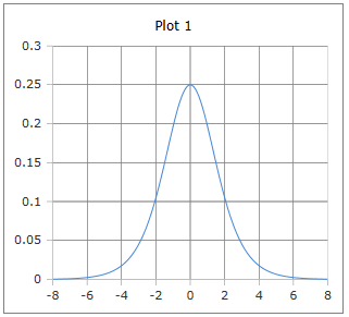
Die glockenförmige Kurve der Sigmoid-Ableitung mit Maximum bei x=0
Die Sigmoid-Ableitung verstehen
Die Ableitung der Sigmoid-Funktion ist von zentraler Bedeutung in der Backpropagation neuronaler Netze. Sie hat eine charakteristische glockenförmige Kurve mit ihrem Maximum bei x=0 und dem Wert 0.25. Die elegante Beziehung σ'(x) = σ(x)·(1-σ(x)) macht die Berechnung besonders effizient, da die Ableitung direkt aus dem Sigmoid-Wert berechnet werden kann.
📉 Grundformeln
Verschiedene Darstellungen:
📊 Eigenschaften
- • Maximum: σ'(0) = 0.25
- • Symmetrisch um x=0
- • Glockenförmige Kurve
- • Schneller Abfall für |x| > 2
🔬 Anwendungen
- • Backpropagation-Algorithmus
- • Gradientenberechnung
- • Optimierung neuronaler Netze
- • Fehler-Rückpropagation
⚠️ Probleme
- • Vanishing Gradient Problem
- • Kleine Werte für |x| > 3
- • Sättigung in tiefen Netzen
- • Begrenzte Lerngeschwindigkeit
Mathematische Herleitung
📉 Ableitung der Sigmoid-Funktion
Schritt-für-Schritt Herleitung:
\[\text{Gegeben: } \sigma(x) = \frac{1}{1 + e^{-x}}\] \[\text{Umschreibung: } \sigma(x) = (1 + e^{-x})^{-1}\] \[\text{Kettenregel anwenden:}\] \[\frac{d\sigma}{dx} = -1 \cdot (1 + e^{-x})^{-2} \cdot \frac{d}{dx}(1 + e^{-x})\] \[= -(1 + e^{-x})^{-2} \cdot (-e^{-x}) = \frac{e^{-x}}{(1 + e^{-x})^2}\]
🔄 Elegante Form herleiten
Umformung zur praktischen Berechnungsform:
\[\sigma'(x) = \frac{e^{-x}}{(1 + e^{-x})^2}\] \[\text{Erweitern mit } e^x:\] \[\sigma'(x) = \frac{e^{-x} \cdot e^x}{(1 + e^{-x})^2 \cdot e^x} = \frac{1}{(1 + e^{-x}) \cdot \frac{(1 + e^{-x})e^x}{e^x}}\] \[= \frac{1}{(1 + e^{-x})} \cdot \frac{1}{\frac{e^x + 1}{e^x}} = \frac{1}{1 + e^{-x}} \cdot \frac{e^x}{e^x + 1}\] \[= \sigma(x) \cdot (1 - \sigma(x))\]
📊 Charakteristische Werte
Wichtige Punkte der Sigmoid-Ableitung:
\[\text{Maximum bei } x = 0: \quad \sigma'(0) = \sigma(0)(1-\sigma(0)) = 0{,}5 \cdot 0{,}5 = 0{,}25\] \[\text{Symmetrie: } \sigma'(-x) = \sigma'(x)\] \[\text{Wendepunkte bei } x = \pm\ln(2+\sqrt{3}) \approx \pm 1{,}317\] \[\text{Grenzwerte: } \lim_{x \to \pm\infty} \sigma'(x) = 0\]
Praktische Berechnungsbeispiele
📝 Beispiel 1: Backpropagation-Schritt
Aufgabe: Gradientenberechnung in neuronaler Schicht
Gegeben: Aktivierung a = σ(2) ≈ 0.881, Fehler δ = 0.15
Berechnung:
\[\text{Sigmoid-Wert: } \sigma(2) = \frac{1}{1 + e^{-2}} \approx 0{,}881\] \[\text{Ableitung: } \sigma'(2) = \sigma(2) \cdot (1 - \sigma(2))\] \[= 0{,}881 \cdot (1 - 0{,}881) = 0{,}881 \cdot 0{,}119 \approx 0{,}105\] \[\text{Gradient: } \frac{\partial E}{\partial z} = \delta \cdot \sigma'(2) = 0{,}15 \cdot 0{,}105 \approx 0{,}016\]
Backpropagation: Dieser Gradient wird für die Gewichtsaktualisierung verwendet
📝 Beispiel 2: Vanishing Gradient Problem
Aufgabe: Gradientenverlauf in tiefen Netzen
Szenario: 5-schichtiges Netzwerk mit extremen Eingaben
Berechnung:
\[\text{Schicht 1: } x_1 = 4 \Rightarrow \sigma'(4) \approx 0{,}018\] \[\text{Schicht 2: } x_2 = 3 \Rightarrow \sigma'(3) \approx 0{,}045\] \[\text{Schicht 3: } x_3 = 2 \Rightarrow \sigma'(2) \approx 0{,}105\] \[\text{Gesamtgradient: } \prod_{i=1}^{3} \sigma'(x_i) = 0{,}018 \cdot 0{,}045 \cdot 0{,}105 \approx 8{,}5 \times 10^{-5}\] \[\text{Problem: Extrem kleine Gradienten in frühen Schichten}\]
Lösung: ReLU-Aktivierungen, Residual Connections, Batch Normalization
📝 Beispiel 3: Optimale Initialisierung
Aufgabe: Xavier/Glorot-Initialisierung verstehen
Ziel: Gradienten in optimaler Größenordnung halten
Berechnung:
\[\text{Optimaler Bereich: } \sigma'(x) > 0{,}1 \Rightarrow |x| < 2{,}2\] \[\text{Xavier-Init: } W \sim \mathcal{N}\left(0, \frac{2}{n_{in} + n_{out}}\right)\] \[\text{Ergebnis: } \sigma'(Wx + b) \text{ bleibt in nutzbarem Bereich}\] \[\text{Vergleich: } \sigma'(0) = 0{,}25 \text{ vs. } \sigma'(3) = 0{,}045\]
Praxis: Gewichte so initialisieren, dass Aktivierungen um 0 bleiben
Backpropagation im Detail
🔄 Gradientenfluß durch Schichten
Rückwärtspropagation mit Sigmoid-Ableitung:
\[\text{Forward Pass: } z^{(l)} = W^{(l)}a^{(l-1)} + b^{(l)}, \quad a^{(l)} = \sigma(z^{(l)})\] \[\text{Backward Pass: } \delta^{(l)} = \frac{\partial E}{\partial z^{(l)}}\] \[\text{Kettenregel: } \delta^{(l-1)} = (W^{(l)})^T \delta^{(l)} \odot \sigma'(z^{(l-1)})\] \[\text{Gewichts-Update: } \frac{\partial E}{\partial W^{(l)}} = \delta^{(l)} (a^{(l-1)})^T\]
📊 Ableitungswerte-Tabelle
| x | σ(x) | σ'(x) | σ'(x)/σ(x) | Gradient-Stärke |
|---|---|---|---|---|
| -3 | 0.047 | 0.045 | 0.953 | Schwach |
| -1 | 0.269 | 0.197 | 0.731 | Mittel |
| 0 | 0.500 | 0.250 | 0.500 | Maximum |
| 1 | 0.731 | 0.197 | 0.269 | Mittel |
| 3 | 0.953 | 0.045 | 0.047 | Schwach |
Moderne Alternativen
🚀 Warum ReLU bevorzugt wird
Vergleich der Ableitungen verschiedener Aktivierungsfunktionen:
\[\text{Sigmoid: } \sigma'(x) = \sigma(x)(1-\sigma(x)) \leq 0{,}25\] \[\text{ReLU: } \text{ReLU}'(x) = \begin{cases} 1 & x > 0 \\ 0 & x < 0 \end{cases}\] \[\text{Leaky ReLU: } \text{LReLU}'(x) = \begin{cases} 1 & x > 0 \\ 0{,}01 & x < 0 \end{cases}\] \[\text{Swish: } \text{Swish}'(x) = \sigma(x) + x \cdot \sigma'(x)\]
Implementierung und Code
💻 Code-Implementierungen
Effiziente Berechnung der Sigmoid-Ableitung:
Python (NumPy):
def sigmoid_derivative(x):
s = sigmoid(x)
return s * (1 - s)
# Wenn sigmoid bereits berechnet:
def sigmoid_derivative_from_output(sigmoid_out):
return sigmoid_out * (1 - sigmoid_out)
# Backpropagation implementieren:
def backward_pass(delta, z):
return delta * sigmoid_derivative(z)
TensorFlow:
# Automatische Differentiation
with tf.GradientTape() as tape:
y = tf.nn.sigmoid(x)
dy_dx = tape.gradient(y, x)
⚡ Optimierte Backpropagation
Praktische Implementation für neuronale Netze:
Vollständige Layer-Implementation:
class SigmoidLayer:
def forward(self, x):
self.output = 1 / (1 + np.exp(-x))
return self.output
def backward(self, grad_output):
# Verwendet gespeicherte Ausgabe
sigmoid_grad = self.output * (1 - self.output)
return grad_output * sigmoid_grad
# Verwendung in Training-Loop:
grad_input = layer.backward(grad_from_above)
💡 Wichtige Eigenschaften der Sigmoid-Ableitung:
- Effizienz: σ'(x) = σ(x)·(1-σ(x)) - berechenbar aus Sigmoid-Wert
- Maximum bei 0: σ'(0) = 0.25 - stärkster Gradient im Nullpunkt
- Symmetrie: Glockenförmige, symmetrische Verteilung
- Vanishing Problem: Kleine Werte für |x| > 2 führen zu schwachen Gradienten
🔬 Anwendungsgebiete der Sigmoid-Ableitung:
- Backpropagation: Grundlage für Gradientenberechnung in NN
- Optimierung: Gewichtsaktualisierung durch Gradientenabstieg
- Fehleranalyse: Verständnis des Vanishing Gradient Problems
- Initialisierung: Design von Xavier/Glorot-Initialisierungsstrategien
acos - Arkuskosinus
acot - Arkuskotangens
acsc - Arkuskosekans
asec - Arkussekans
asin - Arkussinus
atan - Arkustangens
atan2 - Arkustangens von y/x
cos - Kosinus
cot - Kotangens
csc - Kosekans
sec - Sekans
sin - Sinus
sinc - Kardinalsinus
tan - Tangens
hypot - Hypotenuse
deg2rad - Grad in Radiant
rad2deg - Radiant in Grad
Hyperbolik
acosh - Arkuskosinus hyperbolikus
asinh - Areasinus hyperbolikus
atanh - Arkustangens hyperbolikus
cosh - Kosinus hyperbolikus
sinh - Sinus hyperbolikus
tanh - Tangens hyperbolikus
Logarithmus
log - Logarithmus zur angegebene Basis
ln - Natürlicher Logarithmus zur Basis e
log10 - Logarithmus zur Basis 10
log2 - Logarithmus zur Basis 2
exp - Exponenten zur Basis e
Aktivierung
Softmax
Sigmoid
Derivate Sigmoid
Logit
Derivate Logit
Softsign
Derivate Softsign
Softplus
Logistic
Gamma
Eulersche Gamma Funktion
Lanczos Gamma-Funktion
Stirling Gamma-Funktion
Log Gamma-Funktion
Beta
Beta Funktion
Logarithmische Beta Funktion
Unvollstaendige Beta Funktion
Inverse unvollstaendige Beta Funktion
Fehlerfunktionen
erf - Fehlerfunktion
erfc - komplementäre Fehlerfunktion
Kombinatorik
Fakultät
Semifakultät
Steigende Fakultät
Fallende Fakultät
Subfakultät
Permutationen und Kombinationen
Permutation
Kombinationen
Mittlerer Binomialkoeffizient
Catalan-Zahl
Lah Zahl